Part 2: Normalization and background removal

by Morgane Desmau & Marco Alsina

Last update: June 2021

This notebook explains the following steps:

1. Normalization of a spectrum.

2. Background removal of spectrum.

Important: This tutorial assumes you have succesfully completed the previous tutorial in the series: - Part 1: Basics of data processing

# checking version of araucaria and dependencies
from araucaria.utils import get_version
print(get_version(dependencies=True))

Python version      : 3.9.4
Numpy version       : 1.20.3
Scipy version       : 1.6.3
Lmfit version       : 1.0.2
H5py version        : 3.2.1
Matplotlib version  : 3.4.2
Araucaria version   : 0.1.9

1. Retrieving the database filepath

araucaria contains spectra from different beamlines as examples and for testing purposes. The testdata module offers routines to retrieve the respective filepaths.

In this case we will be reading and processing a sample from a minerals database measured at the Fe K-edge in the P65 beamline of DESY, Hamburg (data kindly provided by Morgane Desmau):

1. Fe_database.h5

We will use the get_testpath() function to retrieve the filepath to the database.

# retrieving filepath
from pathlib import Path
from araucaria.testdata import get_testpath

fpath = get_testpath('Fe_database.h5')

# checking that filepath is a Path class
isinstance(fpath, Path)

True

Note

If you prefer to process your own database, just modify the filepath to point to the location of your file.

2. Summarizing a HDF5 database

It is illustrative to first summarize the data contained in an HDF5 database. Here we use the summary_hdf5() function to produce a summary report.

# summarizing database
from araucaria.io import summary_hdf5

report = summary_hdf5(fpath)
report.show()

=================================
id  dataset           mode    n
=================================
1   FeIISO4_20K       mu      5
2   Fe_Foil           mu_ref  5
3   Ferrihydrite_20K  mu      5
4   Goethite_20K      mu      5
=================================

As seen in the report, spectra in the database were acquired in transmission mode (mu), and were merged from at least 5 scans. araucaria also distinguises a reference measurement mu_ref, which is convenient to verify that spectra is properly aligned within a database.

The read_hdf5() function allows us to read a single Group from a HDF5 database. In this case we will read the dataset of ferrous sulfate measured at 20 K.

from araucaria import Group
from araucaria.io import read_hdf5

name  = 'FeIISO4_20K'
group = read_hdf5(fpath, name)

# checking the group class
isinstance(group, Group)

True

3. Spectrum normalization

Analysis and comparison of spectra acquired under different conditions requires normalization. In this regard, XAFS spectra is commonly normalized by setting the absorption edge step to one \((\Delta \mu_0 \sim 1.0)\). Such approach depends on the value of the absorption threshold (\(E_0\)).

The find_e0() function allows to find \(E_0\) for a single scan group:

from araucaria.xas import find_e0

e0 = find_e0(group)
print('e0 value is %1.3f eV' % e0)

e0 value is 7124.723 eV

We can use the previous value to normalize the spectrum and automatically update the group with the pre_edge() function.

Here we use a dictionary to specifiy the normalization parameters, including the pre-edge and post-edge fitting ranges, as well as the coefficients for the pre-edge Victoreen and the post-edge polynomial functions.

Note

We specified the upper end of the post-edge polynomial to be inf. This value defaults to the maximum recorded energy in the scan. Please check the documentation of pre_edge() for further details.

from numpy import inf
from araucaria.xas import pre_edge
from araucaria.plot import fig_pre_edge

# pre-edge parameters
pre_edge_kws = {'pre_range' : [-160, -40],
                'post_range': [150, inf],
                'nvict'     : 2,
                'nnorm'     : 3}

pre_data = pre_edge(group, e0=e0, update=True, **pre_edge_kws)
print('edge step is %1.4f a.u.' % group.edge_step)

edge step is 0.1821 a.u.

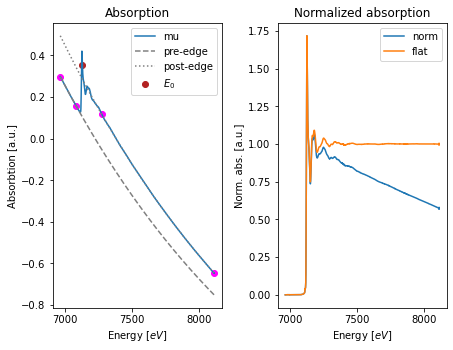
Finally we can plot the normalized spectrum with the fig_pre_edge() function. The function accepts a dictionary of parameters for the figure, so in this case we specify the figure size with the figsize key.

import matplotlib.pyplot as plt

# figure size in inches
fig_kws  = {'figsize' : (6.4, 4.8)}

fig, ax  = fig_pre_edge(group, **fig_kws)
plt.show()

4. Background removal

Once a XAFS spectrum is normalized we can compute the Extended X-ray Fine Structure (EXAFS) \(\chi(k)\). For this we need to remove background signal that accompanies the EXAFS.

araucaria implements background removal with the autobk() function, which accepts a dictionary to provide the parameters. Please check the documentation of autobk() for further details.

from araucaria.xas import autobk

# autobk parameters
autobk_kws = {'rbkg'    : 1.0,
              'k_range' : [0, 14],
              'kweight' : 2,
              'win'     : 'hanning',
              'dk'      : 0.1,
              'nclamp'  : 2,
              'clamp_lo': 1,
              'clamp_hi': 1}

# background removal
autbk_data = autobk(group, update=True, **autobk_kws)

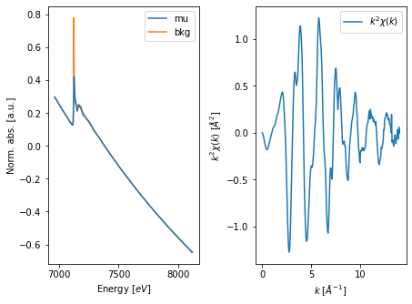
Once we have removed the background signal, we can visualize it along with the \(\chi(k)\) spectrum using the fig_autobk() function. The function also accepts a dictionary of parameters for the figure, provided in this case with the fig_kws dictionary.

# plot background and EXAFS
from araucaria.plot import fig_autobk

fig, ax = fig_autobk(group, show_window=False, **fig_kws)
plt.show()