Part 1: Basics of data processing

by Morgane Desmau & Marco Alsina

Last update: June 2021

The following notebook explains the steps required to create a database in araucaria:

1. Read spectra from files.

2. Align spectra.

3. Merge spectra and calibrate reference channel.

4. Create a database with the processed spectra.

1. Checking version

It is convenient to first check the version of araucaria and its dependencies. In this case we will use the get_version() function.

As seen in the output, this tutorial was developed with version 0.1.9 (your version could vary).

from araucaria.utils import get_version
print(get_version(dependencies=True))

Python version      : 3.9.4
Numpy version       : 1.20.3
Scipy version       : 1.6.3
Lmfit version       : 1.0.2
H5py version        : 3.2.1
Matplotlib version  : 3.4.2
Araucaria version   : 0.1.9

2. Retrieving filepaths

araucaria contains spectra from different beamlines as examples and for testing purposes. The testdata module offers routines to retrieve the respective filepaths.

In this case we will read and process several scans of goethite (an iron oxyhydroxide). Spectra was measured at the Fe K-edge in the P65 beamline of DESY, Hamburg (data kindly provided by Morgane Desmau):

1. 20K_GOE_Fe_K_240.00000.xdi

2. 20K_GOE_Fe_K_240.00001.xdi

3. 20K_GOE_Fe_K_240.00002.xdi

4. 20K_GOE_Fe_K_240.00003.xdi

5. 20K_GOE_Fe_K_240.00004.xdi

We will use the get_testpath() function to construct a list with filepaths to the scan files.

# retrieving filepaths and storing them in a list
from pathlib import Path
from araucaria.testdata import get_testpath

fpaths = []
for i in range(0,5):
    path = get_testpath('20K_GOE_Fe_K_240.0000%i.xdi' % i)
    fpaths.append(path)

# checking that all filepaths are Path classes
all([isinstance(p, Path) for p in fpaths])

True

Note

If you prefer to process your own spectra, just modify the list with filepaths to point to the location of your files.

3. Reading and aligning scans

Once the filepaths have been retrieved we can use the available functions of the io_read module to read them. Since the specra was acquired at the P65 beamline we will be using the read_p65() function:

• For convenience we will read both the transmission and reference channels of each scan file and store it as a Group.

• A single scan (arbitrarily selected) will be used for alignment of the remaining spectra.

• Aligned spectra will be stored together in a Collection.

• A Report is created and its contents printed to stdout.

Alignment will be performed with the align() function. Note that here we explicitly establish an alignment window of -100 eV to 100 eV around the absorption threshold (\(E_0\)) to perform the alignment.

Note

araucaria does not impose a preferred order to approach data pre-processing. Thus, you could also choose to first calibrate a single scan and then align the remaining scans before merging.

from araucaria import Collection
from araucaria.io import read_p65
from araucaria.xas import align, merge

# container of data groups
collection = Collection()

# reading a single scan
ref = read_p65(fpaths[0], scan='mu', ref=True)
collection.add_group(ref, tag='merge')

# reading remaining scans and aligning them
for fpath in fpaths[1:]:
    group = read_p65(fpath, scan='mu', ref=True)
    align(group, ref, window=[-100,100])
    collection.add_group(group, tag='merge')

report = collection.summary(optional=['e_offset'])
report.show()

===========================================================
id  dataset                     tag    mode  n  e_offset
===========================================================
1   20K_GOE_Fe_K_240.00000.xdi  merge  mu    1
2   20K_GOE_Fe_K_240.00001.xdi  merge  mu    1  0.0225
3   20K_GOE_Fe_K_240.00002.xdi  merge  mu    1  0.026688
4   20K_GOE_Fe_K_240.00003.xdi  merge  mu    1  -0.000625
5   20K_GOE_Fe_K_240.00004.xdi  merge  mu    1  0.0064375
===========================================================

Note that each Group dataset is added to the Collection with the add_group() method. This method also allows specification of a tag attribute, which is useful to perform joint operations such as merging spectra. Note that tag attributes are included in the summary report.

Note also that the energy offsets after alignment are negligible, so in this case we could merge the scans without alignment.

Note

If no tag is specified during add_group(), by default the added group will be assigned with tag='scan'.

4. Merging scans

Merge is performed with the merge() function, which accepts a taglistargument to filter which datasets are considered for merging. Since all datasets have the same tag, all are considered for the merge.

# merging scans
report, mgroup = merge(collection, taglist=['merge'], name='20K_GOE_Fe_K')
report.show()

============================================================
id  filename                    mode  e_offset[eV]  e0[eV]
============================================================
1   20K_GOE_Fe_K_240.00000.xdi  mu    0             7126.9
2   20K_GOE_Fe_K_240.00001.xdi  mu    0.0225        7127.2
3   20K_GOE_Fe_K_240.00002.xdi  mu    0.026688      7127
4   20K_GOE_Fe_K_240.00003.xdi  mu    -0.000625     7126.9
5   20K_GOE_Fe_K_240.00004.xdi  mu    0.0064375     7127.2
------------------------------------------------------------
    20K_GOE_Fe_K                mu    0             7126.7
============================================================

5. Calibrating the merged scan

After merging we can verify that the energy of the merged reference channel corresponds to the absorption threshold at the Fe K-edge (7112 eV).

By default the merge() function reports the merge result on the primary channel (transmission in this case): We can verify the energy of the merged reference channels by requesting it explicitly with the option only_mu_ref=True.

# merging only reference scans
report_ref, mgroup_ref = merge(collection, name='20K_GOE_Fe_K_ref', only_mu_ref=True)
report_ref.show()

==============================================================
id  filename                    mode    e_offset[eV]  e0[eV]
==============================================================
1   20K_GOE_Fe_K_240.00000.xdi  mu_ref  0             7111.5
2   20K_GOE_Fe_K_240.00001.xdi  mu_ref  0.0225        7111.4
3   20K_GOE_Fe_K_240.00002.xdi  mu_ref  0.026688      7111.3
4   20K_GOE_Fe_K_240.00003.xdi  mu_ref  -0.000625     7111.2
5   20K_GOE_Fe_K_240.00004.xdi  mu_ref  0.0064375     7111.2
--------------------------------------------------------------
    20K_GOE_Fe_K_ref            mu_ref  0             7111.4
==============================================================

In this case the merge report for the reference channel returns a value of 7111.4 eV, so lets go ahead and calibrate() the merged scan.

After calibration we can verify final value of \(E_0\) with the find_e0() function.

# calibrating and computing e0 for the merged reference scan.
from numpy import allclose
from araucaria.xas import calibrate, find_e0

e0       = 7112    # Fe K-edge
e_offset = calibrate(mgroup, e0, update=True)
e0_ref   = find_e0(mgroup, use_mu_ref=True)

# printing results
print('energy offset of merge: %1.3f eV' % e_offset)
print('e0 of merged reference: %1.1f eV' % e0_ref)
allclose(e0, e0_ref)

energy offset of merge: 0.595 eV
e0 of merged reference: 7112.0 eV

True

6. Plotting merge results

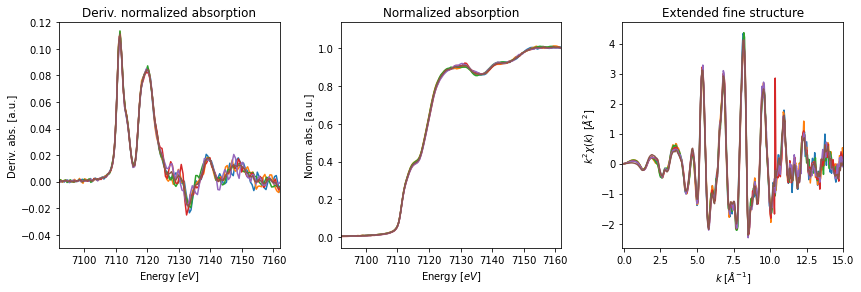
Once the merge is complete, we can provide the merged group and the original collection to the fig_merge() function in order to visualize the results. The function accepts a dictionary to set the parameters for the XAFS figures (fig_pars) as well as a dictionary to set general figure parameters (fig_kws).

Warning

fig_merge() also accepts dictionaries to set the normalization and background removal procedures. However, note that these dictionaries are for visualization and comparison purposes only, and have no effect on the merge itself.

# plot figure of spectra + merge
from araucaria.plot import fig_merge
import matplotlib.pyplot as plt

# general parameters to figure
fig_kws  = {'figsize'  : (12, 4.0)}

# figure parameters for merged reference
fig_pars = {'e_range'  : (e0-20, e0+50),
           'dmu_range' : [-0.05,0.12],
           'k_range'   : [-0.1,15.0],
           'k_mult'    : 2,
           }

# plot of merged reference scans
fig, axes= fig_merge(mgroup_ref, collection, fig_pars=fig_pars, **fig_kws)

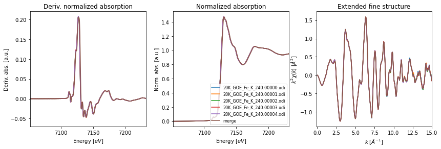
# figure parameters for merged scan
fig_pars = {'e_range'  : (e0-60, e0+120),
           'dmu_range' : [-0.07,0.22],
           'k_range'   : [-0.1,15.0],
           'k_mult'    : 2,
           }

# plot of merged scans
fig, axes= fig_merge(mgroup, collection, fig_pars=fig_pars, **fig_kws)
axes[1].legend(fontsize=8)
plt.show()

7. Saving datasets in an HDF5 database

If we are satisfied with our results, we can save them in a binary format for later retrieval and analysis. The write_collection_hdf5() function allows us to directly save a Collection in the Hierarchical Data Format HDF5.

from araucaria.io import write_collection_hdf5

collection = Collection()
for group in (mgroup, mgroup_ref):
    collection.add_group(group)

# report for collection
report = collection.summary(optional=['merged_scans'])
report.show()

===================================================================
id  dataset           tag   mode    n  merged_scans
===================================================================
1   20K_GOE_Fe_K      scan  mu      5  20K_GOE_Fe_K_240.00000.xdi
                                       20K_GOE_Fe_K_240.00001.xdi
                                       20K_GOE_Fe_K_240.00002.xdi
                                       20K_GOE_Fe_K_240.00003.xdi
                                       20K_GOE_Fe_K_240.00004.xdi
-------------------------------------------------------------------
2   20K_GOE_Fe_K_ref  scan  mu_ref  5  20K_GOE_Fe_K_240.00000.xdi
                                       20K_GOE_Fe_K_240.00001.xdi
                                       20K_GOE_Fe_K_240.00002.xdi
                                       20K_GOE_Fe_K_240.00003.xdi
                                       20K_GOE_Fe_K_240.00004.xdi
===================================================================

# writing collection to HDF5 file
write_collection_hdf5('test_database.h5', collection)

20K_GOE_Fe_K written to test_database.h5.
20K_GOE_Fe_K_ref written to test_database.h5.