Part 4: Linear combination fitting
by Morgane Desmau & Marco Alsina
Last update: June 2021
The following notebook explains the following:
Perform linear combination fitting (LCF) on XANES spectra.
Perform LCF on EXAFS spectra.
Important: This tutorial assumes you have succesfully completed the previous tutorials in the series:
[1]:
# checking version of araucaria and dependencies
from araucaria.utils import get_version
print(get_version(dependencies=True))
Python version      : 3.9.4
Numpy version       : 1.20.3
Scipy version       : 1.6.3
Lmfit version       : 1.0.2
H5py version        : 3.2.1
Matplotlib version  : 3.4.2
Araucaria version   : 0.1.10
1. Accesing the database
In this case we will be reading and processing a minerals database measured at the Fe K-edge in the P65 beamline of DESY, Hamburg (data kindly provided by Morgane Desmau):
Fe_database.h5
We first retrieve the filepath to the database and summarize its contents.
Note
If you prefer to process your own database, just modify the filepath to point to the location of your file.
[2]:
from pathlib import Path
from araucaria.testdata import get_testpath
from araucaria.io import summary_hdf5

# retrieving filepath
fpath = get_testpath('Fe_database.h5')

# summarizing database
report = summary_hdf5(fpath)
report.show()
=================================
id  dataset           mode    n
=================================
1   FeIISO4_20K       mu      5
2   Fe_Foil           mu_ref  5
3   Ferrihydrite_20K  mu      5
4   Goethite_20K      mu      5
=================================
2. Creating a group to fit
We will use the merge() function to create an example signal to fit, in this case a mixture of the 2 original signals from ferrihydrite and goethite minerals.
Note that the original signals are multiplied by normalized amplitude factors to prevent proportions larger than 1 during the fit.
We will store the original signals and the mixture in a Collection, compute normalized spectra through the apply() method, and produce a summary report.
[3]:
from araucaria.io import read_hdf5
from araucaria.xas import merge, pre_edge, autobk
from araucaria import Collection

# name of groups
groupnames = ('Ferrihydrite_20K', 'Goethite_20K')
amp        = [0.5, 0.5]

# initializing collections
collection = Collection()
auxiliary  = Collection()

# reading scans and adding them to collection
for i,name in enumerate(groupnames):
    group = read_hdf5(fpath, name)
    collection.add_group(group, tag='ref')
    group.mu = amp[i]*group.mu
    auxiliary.add_group(group)

# merging scans
report, merge = merge(auxiliary, name='sample')
collection.add_group(merge, tag='scan')

# normalizing spectra in collection
collection.apply(pre_edge)

# printing report
report = collection.summary(optional=['edge_step'])
report.show()
================================================
id  dataset           tag   mode  n  edge_step
================================================
1   Ferrihydrite_20K  ref   mu    5  0.27895
2   Goethite_20K      ref   mu    5  0.4038
3   sample            scan  mu    2  0.34112
================================================
3. Computing expected amplitudes from the LCF
As seen from the summary report, the edge steps of the original signals are not equal. We can compute the expected proportions by re-normalizing the amplitudes considering the proportion of the edge step values:
[4]:
from numpy import sum

edge_steps = report.get_cols(names=['edge_step'], astype='float')[:2]
amplitudes = [amp[i]*val for i, val in enumerate(edge_steps)]
amplitudes = [val/sum(amplitudes) for val in amplitudes]

for i, val in enumerate(amplitudes):
    print('{0:16}: {1:1.3f}'.format(groupnames[i], val))
Ferrihydrite_20K: 0.409
Goethite_20K    : 0.591
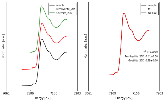
4. Performing XANES LCF
We can perform LCF with the lcf() function. For clarity we use dictionaries to specify the normalization and lcf parameters for the fit. Note that we specify fit_region='xanes' and a fit_range with respect to a fixed absorption threshold in energy units.
Once the LCF is finished we can print a summary with the lcf_report() function.
[5]:
from araucaria.fit import lcf, lcf_report

# parameters for normalization and lcf
k_edge = 7112
pre_edge_kws = {'pre_range' : [-160, -40],
                'post_range': [140, 950],
                'nvict'     : 0,
                'e0'        : k_edge}

lcf_kws      = {'fit_region': 'xanes',
                'sum_one'   : False,
                'fit_range' : [k_edge-20,k_edge+70]}

collection.apply(pre_edge, **pre_edge_kws)
out = lcf(collection, **lcf_kws)
print(lcf_report(out))
[[Parameters]]
    fit_region         = xanes
    fit_range          = [7092, 7182]
    sum_one            = False
[[Groups]]
    scan               = sample
    ref1               = Ferrihydrite_20K
    ref2               = Goethite_20K
[[Fit Statistics]]
    # fitting method   = leastsq
    # function evals   = 10
    # data points      = 168
    # variables        = 2
    chi-square         = 1.5177e-07
    reduced chi-square = 9.1428e-10
    Akaike info crit   = -3494.57580
    Bayesian info crit = -3488.32787
[[Variables]]
    amp1:  0.40894498 +/- 9.9474e-05 (0.02%) (init = 0.5)
    amp2:  0.59225273 +/- 9.9337e-05 (0.02%) (init = 0.5)
[[Correlations]] (unreported correlations are < 0.100)
    C(amp1, amp2) = -1.000
As seen in the report, our prediction for the amplitudes of the original signals is in agreement with the LCF results.
We can visually compare the fitted curve with the original signal with the fig_lcf() function. The plot function accepts a dictionary to set the parameters for the XAFS figures (fig_pars), as well as a dictionary to set general figure parameters (fig_kws).
[6]:
import matplotlib.pyplot as plt
from araucaria.plot import fig_lcf

# figure parameters
offset   = 0.5
fig_kws  = {'figsize'   : (8, 5)}  # size figure
fig_pars = {'e_range'  : (k_edge-50, k_edge+90),
           'e_ticks'   : [k_edge-51, k_edge-3, k_edge+44, k_edge+91],
           'prop_cycle': [{'color'     : ['black', 'red', 'forestgreen'],
                           'linewidth' : [1.5    , 1.5  , 1.5          ],},
                          {'color'     : ['black', 'red', 'grey'],
                           'linewidth' : [1.5    , 1.5  , 1.5   ],}
                         ]}

fig, ax = fig_lcf(out, offset=offset, fig_pars=fig_pars, **fig_kws)
fig.tight_layout()
plt.show()
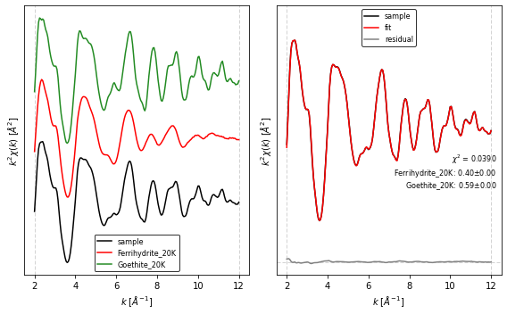
5. Performing EXAFS LCF
The lcf() function also allows LCF of the EXAFS spectrum by specifying the fit_region='exafs'. Note that here we additionally declare a dictionary for the background removal parameters, and modify fit_range to consider values in wavenumber space (\(k\)).
Once the LCF is finished we can print a summary with the lcf_report() function, and plot the resulting fit with the fig_lcf() function.
[7]:
# parameters for normalization, background removal and lcf
k_edge = 7112

autobk_kws   = {'k_range'   : [0, 15],
                'kweight'   : 2,
                'rbkg'      : 1,
                'win'       : 'hanning',
                'dk'        : 0.1,
                'clamp_hi'  : 35}

lcf_kws      = {'fit_region': 'exafs',
                'sum_one'   : False,
                'fit_range'  : [2, 12]}

collection.apply(autobk, **autobk_kws)
out = lcf(collection, **lcf_kws)
print(lcf_report(out))
[[Parameters]]
    fit_region         = exafs
    fit_range          = [2, 12]
    sum_one            = False
    kweight            = 2
[[Groups]]
    scan               = sample
    ref1               = Ferrihydrite_20K
    ref2               = Goethite_20K
[[Fit Statistics]]
    # fitting method   = leastsq
    # function evals   = 10
    # data points      = 201
    # variables        = 2
    chi-square         = 0.03903089
    reduced chi-square = 1.9614e-04
    Akaike info crit   = -1713.88806
    Bayesian info crit = -1707.28145
[[Variables]]
    amp1:  0.40386852 +/- 0.00361482 (0.90%) (init = 0.5)
    amp2:  0.59444931 +/- 0.00300275 (0.51%) (init = 0.5)
[[Correlations]] (unreported correlations are < 0.100)
    C(amp1, amp2) = -0.923
[8]:
# figure parameters
offset   = 2.0
fig_kws  = {'figsize'   : (8, 5)}  # size figure
fig_pars = {'prop_cycle': [{'color'     : ['black', 'red', 'forestgreen'],
                            'linewidth' : [1.5    , 1.5  , 1.5          ]},
                           {'color'     : ['black', 'red', 'grey'],
                            'linewidth' : [1.5    , 1.5  , 1.5   ]}
                          ]}

fig, ax = fig_lcf(out, offset=offset, fig_pars=fig_pars, **fig_kws)
fig.tight_layout()
plt.show()